- Russian Cities Database
- Creating an Interactive Web Map
- Adding a Custom Map Tile
- Setting the Default Map View
- A Map with a Narrower View
- Adding Layers
- Adding Popups
- Circle Markers
- Creating a Color Palette
- Clear the bounds
Interactive Maps with Leaflet Package
Lamova Tamara
18.03.2021
Hello! Today I want to introduce you a leaflet package that used to create interactive maps. Be sure to check out the entire course on Data Camp, which helped me in writing this script. The data for the example was taken from simplemaps, but I will also attach a csv file to this document if you want to reproduce my code.
Russian Cities Database
For this task I have decided to choose Russian cities data set. It contains 723 prominent cities in Russia. Each row includes a city’s latitude, longitude, province and other variables of interest.
library(readr)
ru <- read_csv("ru.csv")
summary(ru)
## city lat lng country
## Length:723 Min. :42.07 Min. : 19.92 Length:723
## Class :character 1st Qu.:49.74 1st Qu.: 38.30 Class :character
## Mode :character Median :54.75 Median : 43.17 Mode :character
## Mean :53.44 Mean : 53.15
## 3rd Qu.:56.65 3rd Qu.: 59.70
## Max. :70.77 Max. :177.52
##
## iso2 admin_name capital population
## Length:723 Length:723 Length:723 Min. : 3188
## Class :character Class :character Class :character 1st Qu.: 32176
## Mode :character Mode :character Mode :character Median : 52004
## Mean : 159931
## 3rd Qu.: 107689
## Max. :17125000
## NA's :97
## population_proper
## Min. : 3188
## 1st Qu.: 32176
## Median : 51768
## Mean : 153412
## 3rd Qu.: 107689
## Max. :13200000
## NA's :97Creating an Interactive Web Map
Using leaflet package in R you can create interactive maps with only a couple of lines of R code. Firstly, let us load the library leaflet and with functions leaflet() and addTiles() create a simple map.
# Load the leaflet library
#install.packages("leaflet")
library(leaflet)
library(dplyr)

# Create a leaflet map with default map tile using addTiles()
leaflet() %>%
    addTiles()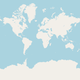
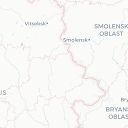
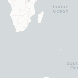
Here addTiles() added the default OpenStreetMap (OSM) tile to your leaflet map. Map tiles weave multiple map images together. The leaflet package have more than 100 map tiles that you can use. These tiles are stored in a list called providers and can be added to your map using addProviderTiles().
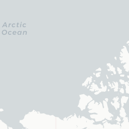
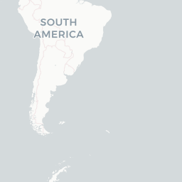
Adding a Custom Map Tile
Map tiles weave multiple map images together. The leaflet package have more than 100 map tiles that you can use. These tiles are stored in a list called providers and can be added to your map using addProviderTiles(). Let’s use Esri map tile as example.
leaflet() %>%
    addProviderTiles("Esri")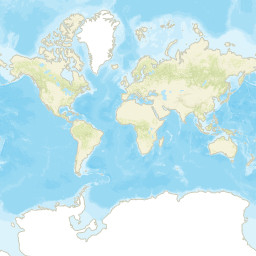
Leaflet | Tiles © Esri
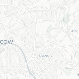
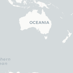
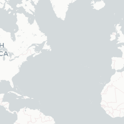
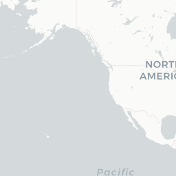
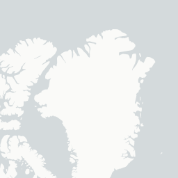
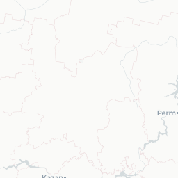
For the next examples I will use CartoDB provider tiles, but feel free to try others.
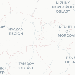
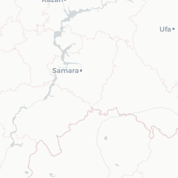
Setting the Default Map View
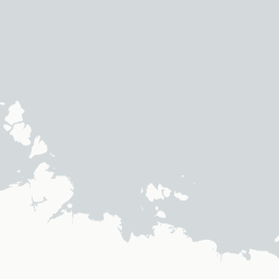
You may have noticed that, by default, maps are zoomed out to the farthest level. Rather than manually zooming and panning, we can load the map centered on a particular point using the setView() function.
setView() takes three numeric arguments:
- lng (not “lon” or “long”)
- lat
- zoom
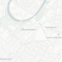
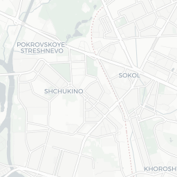
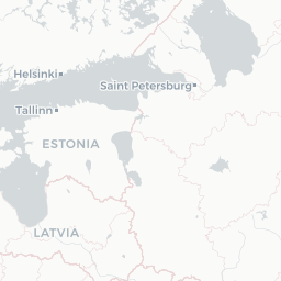
Let us use the coordinates from our data set to create a map with the “CartoDB” provider tile that is centered on Moscow with a zoom of 6.
head(ru, 1)| city | lat | lng | country | iso2 | admin_name | capital | population | population_proper |
|---|---|---|---|---|---|---|---|---|
| Moscow | 55.7558 | 37.6178 | Russia | RU | Moskva | primary | 17125000 | 13200000 |
leaflet()  %>%
    addProviderTiles("CartoDB")  %>%
    setView(lng = 37.6178, lat = 55.7558, zoom = 6)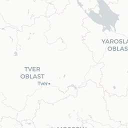
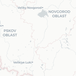
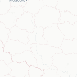
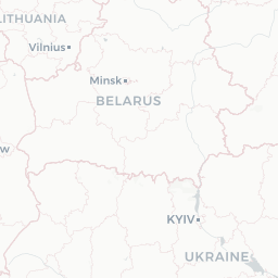
A Map with a Narrower View
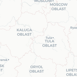
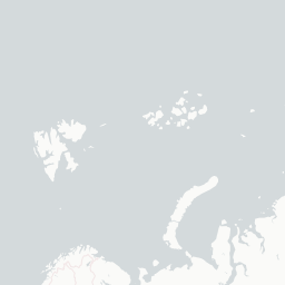
What if we want to limit the ability to move around the map? This can be done using the options argument in the leaflet() function. By setting minZoom and dragging (dragging = FALSE), we can create an interactive web map that will always focus on a specific area.
Moreover, if we want users to be able to drag the map while ensuring that they do not stray too far, we can set the maps maximum boundaries.
Let us use maximum bounds of .05 decimal degrees from the Moscow and minzoom 12.
leaflet(options = leafletOptions(
                    # Set minZoom and dragging
                    minZoom = 12, dragging = TRUE)) %>%
  addProviderTiles("CartoDB") %>%

  # Set default zoom level
  setView(lng = 37.6178, lat = 55.7558, zoom = 12) %>%

  # Set max bounds of map
  setMaxBounds(lng1 = 37.6178 + .05,
               lat1 = 55.7558 + .05,
               lng2 = 37.6178 - .05,
               lat2 = 55.7558 - .05)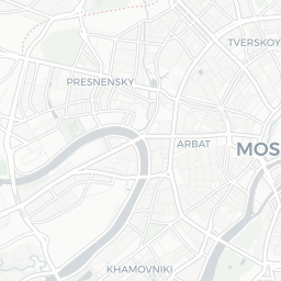
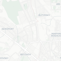
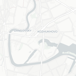
Now we cannot move further than 0.5 degrees from Moscow.
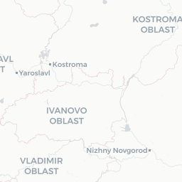
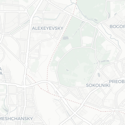
Adding Layers
One of the most common layers to add to a leaflet map is location markers, using addTiles() or addProviderTiles() into the add markers function.
For example, if we plot Moscow by passing the coordinates to addMarkers() as numeric vectors with one element, our web map will place a blue drop pin at the coordinate. We can also plot several cities.
In our data set, we have variable capital. It can be:
- primary - country’s capital (e.g. Moscow)
- admin - first-level admin capital (e.g. Samara)
- minor - lower-level admin capital (e.g. Anapa)
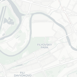
Let us try to plot all first-level admin capitals and add layers to it.
# Plot Moscow with zoom of 12
#leaflet() %>%
    #addProviderTiles("CartoDB") %>%
    #addMarkers(lng = 37.6178, lat = 55.7558)  %>%
#setView(lng = 37.6178, lat = 55.7558, zoom = 12)# Plot first-level admin capitals' locations
ru_admin = ru %>% filter(capital == "admin")
leaflet() %>%
addProviderTiles("CartoDB") %>%
addMarkers(lng = ru_admin$lng, lat = ru_admin$lat)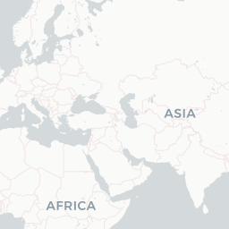


Adding Popups
To make a map more informative we can add popups by specifying the popup argument in the addMarkers() function. Firstly we store it in an object. Then we can pipe this object into functions.
# Store leaflet hq map in an object called map
map <- leaflet() %>%
          addProviderTiles("CartoDB") %>%
          # Use dc_hq to add the hq column as popups
          addMarkers(lng = ru$lng[1], lat = ru$lat[1],
                     popup = ru$city[1])

# Center the view of map on the Moscow with a zoom of 5
map_zoom <- map %>%
      setView(lng = 37.6178, lat = 55.7558,
              zoom = 5)

# Print map_zoom
map_zoom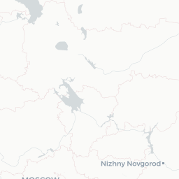
Circle Markers
Circle markers are notably different from pin markers:
- We can control their size
- They do not “stand-up” on the map
- We can more easily change their color
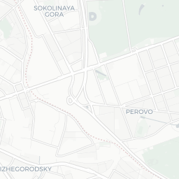
We can add it using function addCircleMarkers().
# Use addCircleMarkers() to plot each first-level admin capitals as a circle
map2 <- leaflet() %>%
          addProviderTiles("CartoDB") %>%
    addCircleMarkers(lng = ru_admin$lng, lat = ru_admin$lat)

map2Changing their size and color and add markers as we did before.
# Change the radius of each circle to be 2 pixels and the color to red
map1 <- leaflet() %>%
          addProviderTiles("CartoDB") %>%
  addCircleMarkers(lng = ru_admin$lng, lat = ru_admin$lat,
                     radius = 2, color = "yellow")

map1Creating a Color Palette
With colorFactor() we can create a color palette that maps colors the levels of a factor variable. Let’s create a map coloring different types of cities.
# Make a color palette called pal for the values of `capital` using `colorFactor()`
# Colors: "red", "blue", and "#9b4a11" for "capital", "admin", and "minor" cities, respectively
pal <- colorFactor(palette = c("red", "blue", "yellow"),
                   levels = c("primary", "admin", "minor"))

ru1 <- ru %>% filter(capital == "primary" | capital == "admin" | capital == "minor")

# Add circle markers that color colleges using pal() and the values of capital
map3 <- leaflet() %>%
          addProviderTiles("CartoDB") %>%
  addCircleMarkers(data = ru1, radius = 2, popup = ~city) %>%
  addCircleMarkers(data = ru1, radius = 2,
                         color = ~pal(capital),
                         label = ~paste0(city, " (", capital, ")"))


# Add a legend that displays the colors used in pal
map3 %>%
    addLegend(pal = pal,
values = c("primary", "admin", "minor"))Now you see maps with Russian cities and their types of capital.
Clear the bounds
Finally, if you do not want to create multiple maps in your environment, just clean the bounds.
map3 <- map %>%
            clearMarkers() %>%
            clearBounds()