Eigenvector Centrality

A natural extension of degree centrality is eigenvector centrality. In-degree centrality awards one centrality point for every link a node receives. But not all vertices are equivalent: some are more relevant than others, and, reasonably, endorsements from important nodes count more. The eigenvector centrality thesis reads:

A node is important if it is linked to by other important nodes.

Eigenvector centrality differs from in-degree centrality: a node receiving many links does not necessarily have a high eigenvector centrality (it might be that all linkers have low or null eigenvector centrality). Moreover, a node with high eigenvector centrality is not necessarily highly linked (the node might have few but important linkers).

Eigenvector centrality, regarded as a ranking measure, is a remarkably old method. Early pioneers of this technique are Wassily W. Leontief (The Structure of American Economy, 1919-1929. Harvard University Press, 1941) and John R. Seeley (The net of reciprocal influence: A problem in treating sociometric data. The Canadian Journal of Psychology, 1949). Read the full story full story.

Math

Let

A = (a_{i, j})

$A = (a_{i,j})$ be the adjacency matrix of a graph. The eigenvector centrality

x_{i}

$x_{i}$ of node

i

$i$ is given by:

x_{i} = \frac{1}{λ} \sum_{k} a_{k, i} x_{k}

$x_i = \frac{1}{\lambda} \sum_k a_{k,i} \, x_k$ where

λ \neq 0

$\lambda \neq 0$ is a constant. In matrix form we have:

λ x = x A

$\lambda x = x A$

Hence the centrality vector

x

$x$ is the left-hand eigenvector of the adjacency matrix

A

$A$ associated with the eigenvalue

λ

$\lambda$ . It is wise to choose

λ

$\lambda$ as the largest eigenvalue in absolute value of matrix

A

$A$ . By virtue of Perron-Frobenius theorem, this choice guarantees the following desirable property: if matrix

A

$A$ is irreducible, or equivalently if the graph is (strongly) connected, then the eigenvector solution

x

$x$ is both unique (up to a multiplicative constant) and positive.

The power method can be used to solve the eigenvector centrality problem. Let $m(v)$ denote the signed component of maximal magnitude of vector $v$ . If there is more than one maximal component, let $m(v)$ be the first one. For instance, $m(-3,3,2) = -3$ . Let $x^{(0)} = e$ , where $e$ is the vector of all 1's. For $k \geq 1$ :

repeatedly compute $x^{(k)} = x^{(k-1)} A$ ;
normalize $x^{(k)} = x^{(k)} / m(x^{(k)})$ ;

until the desired precision is achieved. It follows that $x^{(k)}$ converges to the dominant eigenvector of $A$ and $m(x^{(k)})$ converges to the dominant eigenvalue of $A$ . If matrix $A$ is sparse, each vector-matrix product can be performed in linear time in the size of the graph.

Let

| λ_{1} | \geq | λ_{2} | \dots \geq | λ_{n} |

A

$A$ . The power method converges if

| λ_{1} | > | λ_{2} |

$|\lambda_1| > |\lambda_2|$ . The rate of convergence is the rate at which

(λ_{2} / λ_{1})^{k}

$(\lambda_2 / \lambda_1)^k$ goes to

0

$0$ . Hence, if the sub-dominant eigenvalue is small compared to the dominant one, then the method quickly converges. If

A

$A$ is a symmetric matrix, that is the graph of

A

$A$ is undirected, then the eigenvalues of

A

$A$ are all real numbers (in general, they might be complex numbers). In this case, it holds that the graph of

A

$A$ is bipartite if and only if

λ_{1}

$\lambda_1$ and

- λ_{1}

$-\lambda_1$ are eigenvalues of

A

$A$ . Hence, for bipartite graphs

λ_{2} = - λ_{1}

$\lambda_2 = - \lambda_1$ and hence

| λ_{1} | = | λ_{2} |

$|\lambda_1| = |\lambda_2|$ . It follows that the power method diverges on bipartite graphs. Lanczos and Jacobi-Davidson methods are faster alternatives to power method that converge also on bipartite graphs.

Code

The built-in function eigen_centrality (R) computes eigenvector centrality (using ARPACK package).

A user-defined function eigenvector.centrality follows:


# Eigenvector centrality (direct method)
#INPUT
# g = graph
# t = precision
# OUTPUT
# A list with:
# vector = centrality vector
# value = eigenvalue
# iter = number of iterations

eigenvector.centrality = function(g, t=6) {
  A = as_adjacency_matrix(g, sparse=FALSE);
  n = vcount(g);
  x0 = rep(0, n);
  x1 = rep(1/n, n);
  eps = 1/10^t;
  iter = 0;
  while (sum(abs(x0 - x1)) > eps) {
    x0 = x1;
    x1 = x1 %*% A;
    m = x1[which.max(abs(x1))];
    x1 = x1 / m;
    iter = iter + 1;
  } 
  return(list(vector = as.vector(x1), value = m, iter = iter))
}

Example

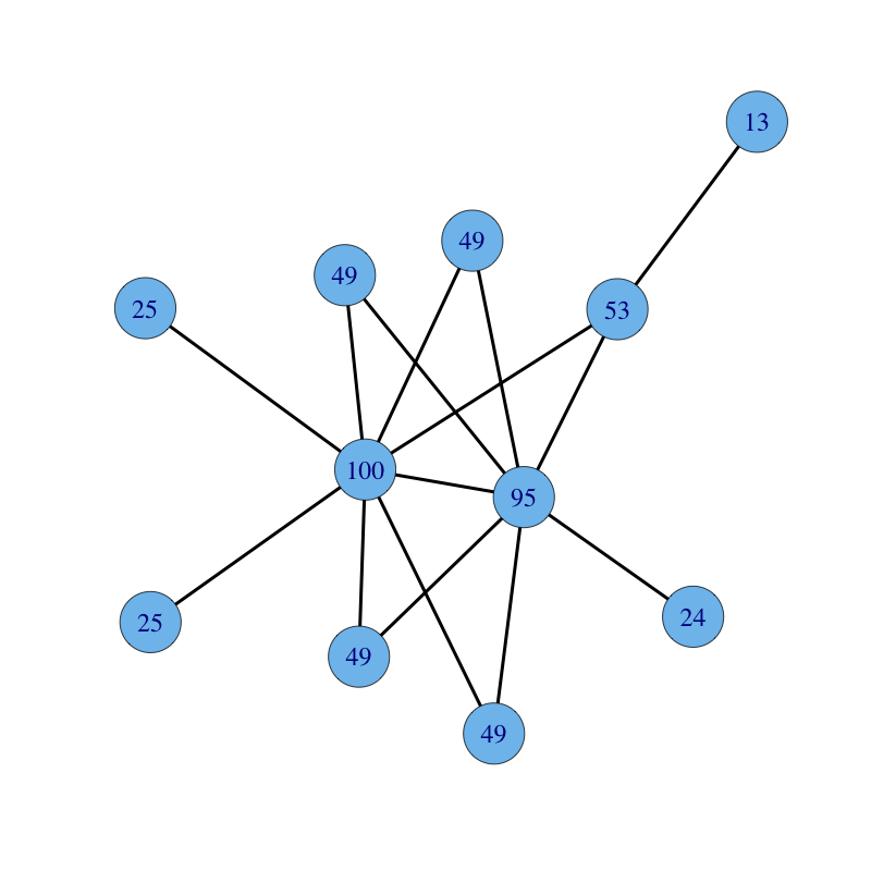
An undirected connected graph with nodes labelled with their eigenvector centrality follows: