3 Jednosmjerna analiza varijance
Neka uvodna priča… 1
PDF od F-distribucije
Fdist <- expand_grid(d1 = c(1,2,5,10,15,50), d2 = c(1,2,5,10,15,50)) %>%
  group_by(d1,d2) %>%
  summarize(x = seq(0,5,0.01), fun = df(x, df1 = d1, df2 = d2), .groups = "drop")
Fdist %>%
  ggplot(aes(x = x, y = fun)) +
  geom_line(color = "blue") + ylim(0,2.5) +
  ylab("df(x)") + facet_grid(vars(d1), vars(d2), labeller = label_both)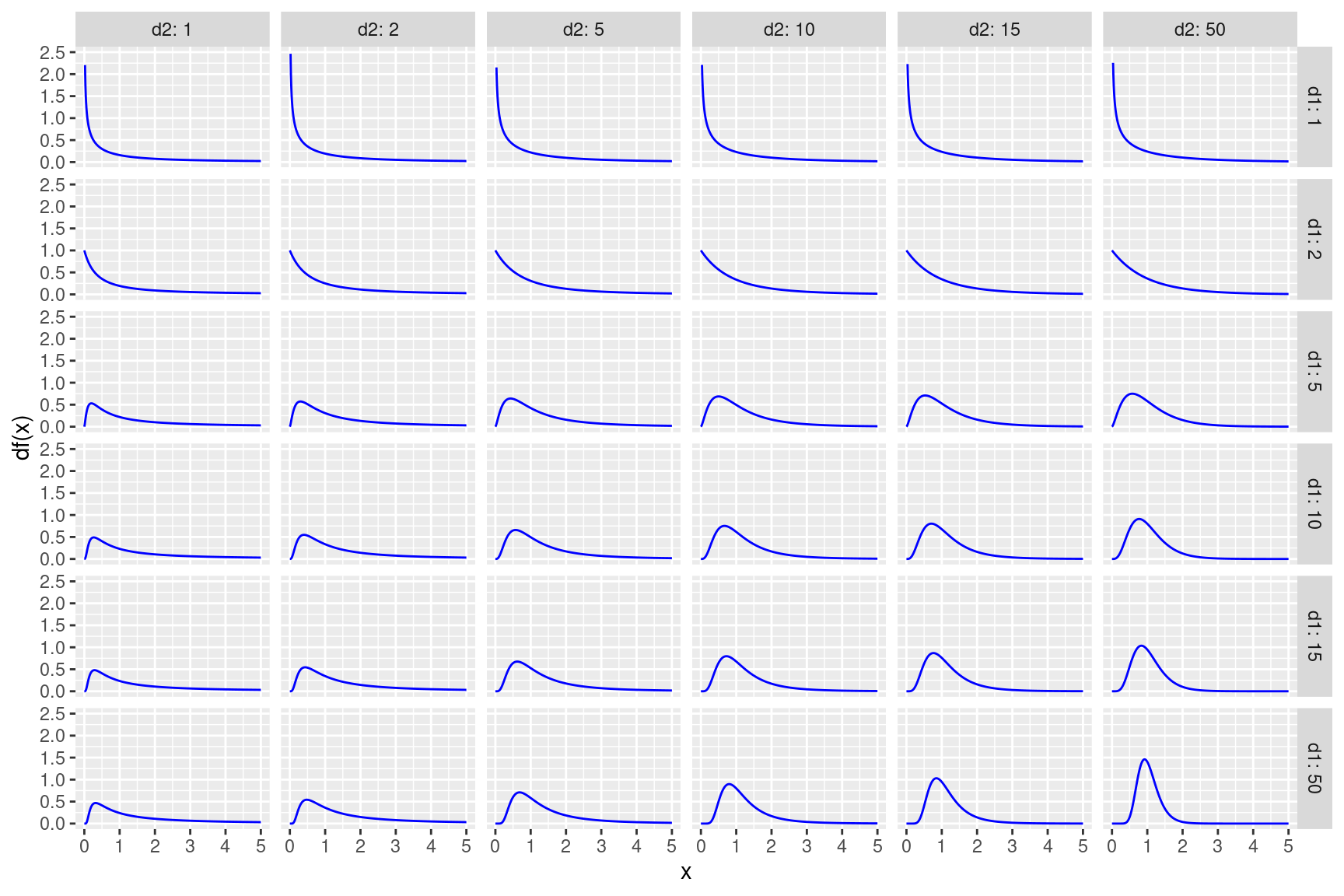
Figure 3.1: F-distribucije s različitim stupnjevima slobode
3.1 Malo matematike
Neka je \(x_{ij}\) \(j\)-to opažanje u \(i\)-toj grupi, \(\bar{x}_i\) aritmetička sredina \(i\)-te grupe i \(\bar{x}\) aritmetička sredina svih opažanja. Tada je \[x_{ij}=\bar{x}+(\bar{x}_i-\bar{x})+(x_{ij}-\bar{x}_i)\] pri čemu je \(\bar{x}_i-\bar{x}\) odstupanje aritmetičke sredine \(i\)-te grupe od aritmetičke sredine svih opažanja, a \(x_{ij}-\bar{x}_i\) odstupanje \(j\)-tog opažanja iz \(i\)-te grupe od aritmetičke sredine te grupe.
Neka je \(m\) ukupni broj grupa, a \(n_i\) broj opažanja u \(i\)-toj grupi. Varijacije unutar grupa računaju se po formuli \[SSD_W=\sum_{i=1}^{m}{\sum_{j=1}^{n_i}{(x_{ij}-\bar{x}_i)^2}},\] a varijacije između grupa po formuli \[SSD_B=\sum_{i=1}^{m}{n_i(\bar{x}_{i}-\bar{x})^2}.\]
3.2 Primjer
ToothGrowth$dose <- factor(ToothGrowth$dose)
a1_model <- aov(len ~ dose, data = ToothGrowth)
print(summary(a1_model), digits = 7)
## Df Sum Sq Mean Sq F value Pr(>F)
## dose 2 2426.434 1213.2172 67.41574 9.5327e-16 ***
## Residuals 57 1025.775 17.9961
## ---
## Signif. codes: 0 '***' 0.001 '**' 0.01 '*' 0.05 '.' 0.1 ' ' 1Ručni izračun
Ybar <- mean(ToothGrowth$len)
tablica <- ToothGrowth %>% group_by(dose) %>%
  mutate(Yk = mean(len), Nk = n()) %>% ungroup()
SSB <- tablica %>% summarize(SSB = sum((Yk - Ybar)^2)) %>% pull(SSB)
SSW <- tablica %>% summarize(SSW = sum((len - Yk)^2)) %>% pull(SSW)
dfB <- nlevels(factor(ToothGrowth$dose)) - 1
dfW <- nrow(tablica) - nlevels(factor(ToothGrowth$dose))
MSB <- SSB / dfB
MSW <- SSW / dfW
Fvalue <- MSB / MSW
pvalue <- pf(Fvalue, dfB, dfW, lower.tail = FALSE)
list(SSB = SSB, SSW = SSW, dfB = dfB, dfW = dfW, MSB = MSB,
     MSW = MSW, Fvalue = Fvalue, pvalue = pvalue)
## $SSB
## [1] 2426.434
##
## $SSW
## [1] 1025.775
##
## $dfB
## [1] 2
##
## $dfW
## [1] 57
##
## $MSB
## [1] 1213.217
##
## $MSW
## [1] 17.99605
##
## $Fvalue
## [1] 67.41574
##
## $pvalue
## [1] 9.532727e-16tibble(x = seq(1,40,0.01)) %>%
ggplot(aes(x)) +
geom_text(aes(x=Fvalue, label="F", y=0.1), nudge_x = 0.9, colour="red",
text=element_text(size=11)) +
geom_area(stat = "function", fun = df, args = list(df1 = dfB, df2 = dfW), fill = "pink",
xlim = c(qf(0.95, df1 = dfB, df2 = dfW), 40), alpha=0.75) +
geom_vline(xintercept = Fvalue, linetype = "dotted") +
stat_function(fun=df, args = list(df1 = dfB, df2 = dfW), color="blue", xlim=c(1,40)) +
labs(title = "one way ANOVA")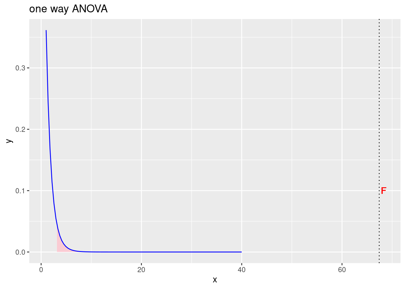
Figure 3.2: Prihvaćamo alternativnu hipotezu da postoji značajna razlika srednjih vrijednosti po grupama
Effect size
Trebamo učitati paket lsr.
library(lsr)Nakon toga možemo koristiti funkciju etaSquared.
etaSquared(x = a1_model)## eta.sq eta.sq.part
## dose 0.7028642 0.7028642Isti rezultat možemo dobiti i ručnim izračunom.
SSB / (SSB + SSW) ## [1] 0.70286423.3 Post hoc tests
pairwise.t.test( x = ToothGrowth$len, g = ToothGrowth$dose, p.adjust.method = "none")##
## Pairwise comparisons using t tests with pooled SD
##
## data: ToothGrowth$len and ToothGrowth$dose
##
## 0.5 1
## 1 6.7e-09 -
## 2 < 2e-16 1.4e-05
##
## P value adjustment method: nonepairwise.t.test( x = ToothGrowth$len, g = ToothGrowth$dose,
p.adjust.method = "bonferroni")##
## Pairwise comparisons using t tests with pooled SD
##
## data: ToothGrowth$len and ToothGrowth$dose
##
## 0.5 1
## 1 2.0e-08 -
## 2 4.4e-16 4.3e-05
##
## P value adjustment method: bonferronipairwise.t.test( x = ToothGrowth$len, g = ToothGrowth$dose, p.adjust.method = "holm")##
## Pairwise comparisons using t tests with pooled SD
##
## data: ToothGrowth$len and ToothGrowth$dose
##
## 0.5 1
## 1 1.3e-08 -
## 2 4.4e-16 1.4e-05
##
## P value adjustment method: holmTukeyHSD(a1_model)## Tukey multiple comparisons of means
## 95% family-wise confidence level
##
## Fit: aov(formula = len ~ dose, data = ToothGrowth)
##
## $dose
## diff lwr upr p adj
## 1-0.5 9.130 5.901805 12.358195 0.00e+00
## 2-0.5 15.495 12.266805 18.723195 0.00e+00
## 2-1 6.365 3.136805 9.593195 4.25e-053.4 Levene test
Trebamo najprije učitati paket car.
library(car)Nakon toga možemo koristiti funkciju leveneTest za ispitivanje homogenosti varijanci po grupama.
leveneTest(a1_model, center = mean)## Levene's Test for Homogeneity of Variance (center = mean)
## Df F value Pr(>F)
## group 2 0.7328 0.485
## 57Zapravo, Levene test radi anovu na varijabli \(Z\) koja je definirana s \(z_{ik}=|x_{ik}-\bar{x}_k|\).
tablica1 <- tablica %>% mutate(Zk = abs(len - Yk))
tablica1
## # A tibble: 60 × 6
## len supp dose Yk Nk Zk
## <dbl> <fct> <fct> <dbl> <int> <dbl>
## 1 4.2 VC 0.5 10.605 20 6.405
## 2 11.5 VC 0.5 10.605 20 0.895
## 3 7.3 VC 0.5 10.605 20 3.305
## 4 5.8 VC 0.5 10.605 20 4.805
## 5 6.4 VC 0.5 10.605 20 4.205
## 6 10 VC 0.5 10.605 20 0.60500
## 7 11.2 VC 0.5 10.605 20 0.59500
## 8 11.2 VC 0.5 10.605 20 0.59500
## 9 5.2 VC 0.5 10.605 20 5.405
## 10 7 VC 0.5 10.605 20 3.605
## # … with 50 more rowshom <- aov(Zk ~ dose, data = tablica1)
print(summary(hom), digits = 7)## Df Sum Sq Mean Sq F value Pr(>F)
## dose 2 8.8526 4.426282 0.73277 0.48505
## Residuals 57 344.3092 6.0405133.5 Normalnost reziduala
a1.residuals <- tibble(res = residuals(object = a1_model))
a1.residuals
## # A tibble: 60 × 1
## res
## <dbl>
## 1 -6.4050
## 2 0.89500
## 3 -3.3050
## 4 -4.805
## 5 -4.2050
## 6 -0.60500
## 7 0.59500
## 8 0.59500
## 9 -5.4050
## 10 -3.6050
## # … with 50 more rowsHistogram
ggplot(a1.residuals, aes(x=res)) + geom_histogram(binwidth=1, fill="pink", color="red")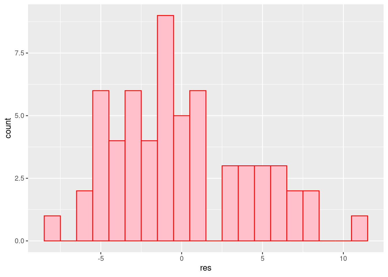
QQ-plot
ggplot(a1.residuals, aes(sample = res)) + stat_qq() + stat_qq_line()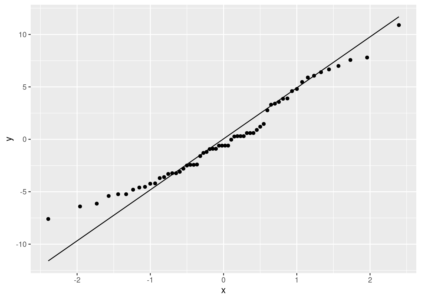
Shapiro-Wilk test za ispitivanje normalnosti
Početna hipoteza: “Populacija ima normalnu distribuciju.”
shapiro.test(a1.residuals$res)##
## Shapiro-Wilk normality test
##
## data: a1.residuals$res
## W = 0.96731, p-value = 0.10763.6 Welchova ANOVA
Koristi se kada nije zadovoljen uvjet homogenosti varijanci grupa.
oneway.test(len ~ dose, data = ToothGrowth)##
## One-way analysis of means (not assuming equal variances)
##
## data: len and dose
## F = 68.401, num df = 2.000, denom df = 37.743, p-value = 2.812e-13Ako stavimo var.equal = TRUE, dobivamo standardnu 1-ANOVU.
oneway.test(len ~ dose, data = ToothGrowth, var.equal = TRUE)##
## One-way analysis of means
##
## data: len and dose
## F = 67.416, num df = 2, denom df = 57, p-value = 9.533e-16Ručni izračun
shap <- ToothGrowth %>% group_by(dose) %>%
  summarize(Xk = mean(len), v = var(len), n = n(), w = n / v)
J <- nlevels(ToothGrowth$dose)
U <- shap %>% summarize(U = sum(w)) %>% pull(U)
Xtilda <- shap %>% summarize(Xtilda = 1 / U * sum(w * Xk)) %>% pull(Xtilda)
A <- shap %>%
  summarize(A = 1 / (J - 1) * sum(w * (Xk - Xtilda)^2)) %>%
  pull(A)
B <- shap %>%
  summarize(B = 2 * (J - 2) / (J^2 - 1) * sum((1 - w / U)^2 / (n - 1))) %>%
  pull(B)
Fw <- A / (1+ B)
v1 <- J - 1
v2 <- shap %>%
  summarize(v2 = (J^2 - 1) / (3 * sum((1 - w / U)^2 / (n - 1)))) %>%
  pull(v2)
pvalue <- pf(Fw, df1=v1, df2=v2, lower.tail = FALSE)
list(tablica = shap, U = U, Xtilda = Xtilda, A = A, B = B, Fw = Fw,
     df1 = v1, df2 = v2, pvalue = pvalue)
## $tablica
## # A tibble: 3 × 5
## dose Xk v n w
## <fct> <dbl> <dbl> <int> <dbl>
## 1 0.5 10.605 20.248 20 0.98776
## 2 1 19.735 19.496 20 1.0258
## 3 2 26.1 14.244 20 1.4041
##
## $U
## [1] 3.417685
##
## $Xtilda
## [1] 19.71122
##
## $A
## [1] 69.60916
##
## $B
## [1] 0.0176632
##
## $Fw
## [1] 68.40098
##
## $df1
## [1] 2
##
## $df2
## [1] 37.74325
##
## $pvalue
## [1] 2.812385e-133.7 Kruskal-Wallis test
Koristi se kada nije zadovoljen uvjet normalnosti.
kruskal.test(len ~ dose, data = ToothGrowth)##
## Kruskal-Wallis rank sum test
##
## data: len by dose
## Kruskal-Wallis chi-squared = 40.669, df = 2, p-value = 1.475e-09Ručni izračun
tooth.rank <- ToothGrowth %>% mutate(Rk = rank(len))
kw.tab <- tooth.rank %>% group_by(dose) %>%
  summarize(Rkbar = mean(Rk), Nk = n()) %>% ungroup()
Rbar <- mean(tooth.rank$Rk)
RSS.tot <- tooth.rank %>% summarize(RSS.tot = sum((Rk - Rbar)^2)) %>% pull(RSS.tot)
RSS.b <- kw.tab %>% summarize(RSS.b = sum(Nk * (Rkbar - Rbar)^2)) %>% pull(RSS.b)
N <- sum(kw.tab$Nk)
K <- (N - 1) * RSS.b / RSS.tot
dfB <- nlevels(tooth.rank$dose) - 1
pvalue <- pchisq(K, dfB, lower.tail = FALSE)
list(RSS.tot = RSS.tot, RSS.b = RSS.b, dfB = dfB,
     K = K, pvalue = pvalue)
## $RSS.tot
## [1] 17981
##
## $RSS.b
## [1] 12394.38
##
## $dfB
## [1] 2
##
## $K
## [1] 40.66894
##
## $pvalue
## [1] 1.475207e-09tibble(x = seq(0,50,0.01)) %>%
ggplot(aes(x)) +
geom_text(aes(x=K, label="K", y=0.1), nudge_x = 0.9, colour="red",
text=element_text(size=11)) +
geom_area(stat = "function", fun = dchisq, args = list(df = dfB), fill = "pink",
xlim = c(qchisq(0.95, df = dfB), 40), alpha=0.75) +
geom_vline(xintercept = K, linetype = "dotted") +
stat_function(fun=dchisq, args = list(df = dfB), color="blue", xlim=c(0,50)) +
labs(title = "Kruskal-Wallis test")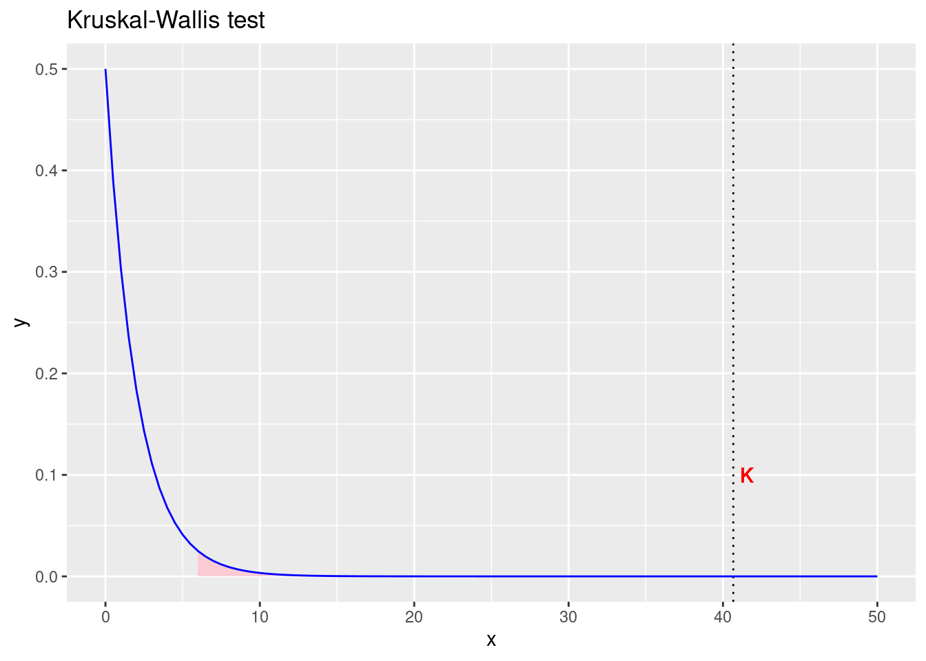
Figure 3.3: Prihvaćamo alternativnu hipotezu da postoji značajna razlika srednjih vrijednosti po grupama
Dunn test (post hoc test)
Link
Dunn test
library(FSA)dunnTest(len ~ dose, data=ToothGrowth, method="bonferroni")## Dunn (1964) Kruskal-Wallis multiple comparison## p-values adjusted with the Bonferroni method.## Comparison Z P.unadj P.adj
## 1 0.5 - 1 -3.554911 3.781068e-04 1.134321e-03
## 2 0.5 - 2 -6.362612 1.983517e-10 5.950552e-10
## 3 1 - 2 -2.807701 4.989660e-03 1.496898e-02library(dunn.test)
dunn.test(ToothGrowth$len, ToothGrowth$dose, altp = TRUE, table = FALSE, list = TRUE)## Kruskal-Wallis rank sum test
##
## data: x and group
## Kruskal-Wallis chi-squared = 40.6689, df = 2, p-value = 0
##
##
## Comparison of x by group
## (No adjustment)
##
## List of pairwise comparisons: Z statistic (p-value)
## -----------------------------
## 0.5 - 1 : -3.554911 (0.0004)*
## 0.5 - 2 : -6.362611 (0.0000)*
## 1 - 2 : -2.807700 (0.0050)*
##
## alpha = 0.05
## Reject Ho if p <= alphalibrary(dunn.test)
dunn.test(ToothGrowth$len, ToothGrowth$dose, table = FALSE, list = TRUE)## Kruskal-Wallis rank sum test
##
## data: x and group
## Kruskal-Wallis chi-squared = 40.6689, df = 2, p-value = 0
##
##
## Comparison of x by group
## (No adjustment)
##
## List of pairwise comparisons: Z statistic (p-value)
## -----------------------------
## 0.5 - 1 : -3.554911 (0.0002)*
## 0.5 - 2 : -6.362611 (0.0000)*
## 1 - 2 : -2.807700 (0.0025)*
##
## alpha = 0.05
## Reject Ho if p <= alpha/2samo primjer za fusnotu :)↩︎