2 t-test

Koristila se literatura (Navarro 2015), …

PDF od t-distribucije

tablica <- tibble(sn =c(2,3,4,5,6,7,10,15,20,30,40,50)) %>% group_by(sn) %>%
  summarize(x = seq(-4,4,0.01), fun = dt(x, df = sn), 
            gauss = dnorm(x), .groups = "drop")
tablica %>%
  ggplot(aes(x = x)) + 
  geom_line(aes(y=fun), color = "blue") +
  geom_line(aes(y=gauss), linetype="dashed") +
  ylab("PDF(x)") + facet_wrap(~sn)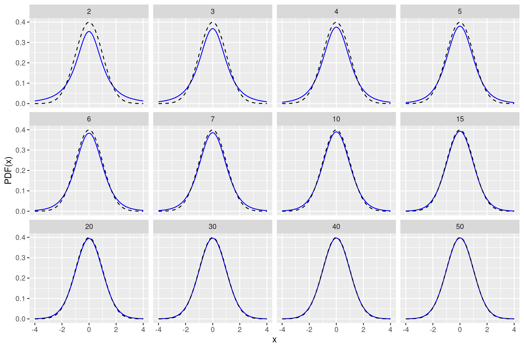

Figure 2.1: t-distribucija s različitim stupnjevima slobode i standardna normalna distribucija

Primjer
The response is the length of odontoblasts (cells responsible for tooth growth) in 60 guinea pigs. Each animal received one of three dose levels of vitamin C (0.5, 1, and 2 mg/day) by one of two delivery methods, orange juice or ascorbic acid (a form of vitamin C and coded as VC).

options(pillar.sigfig=5)
data("ToothGrowth")
glimpse(ToothGrowth)

## Rows: 60
## Columns: 3
## $ len  <dbl> 4.2, 11.5, 7.3, 5.8, 6.4, 10.0, 11.2, 11.2, 5.2, 7.0, 16.5, 16.5,…
## $ supp <fct> VC, VC, VC, VC, VC, VC, VC, VC, VC, VC, VC, VC, VC, VC, VC, VC, V…
## $ dose <dbl> 0.5, 0.5, 0.5, 0.5, 0.5, 0.5, 0.5, 0.5, 0.5, 0.5, 1.0, 1.0, 1.0, …

2.1 One sample t-test for a hypothesized mean

Question: Is the mean of a sample significantly different from a hypothesized mean?

When to use the test? You want to compare the sample mean to a hypothesized value. The test assumes the sample observations are normally distributed and the population standard deviation is unknown.

Dvosmjerni t-test
Početna hipoteza: $\mu=19$
Alternativna hipoteza: $\mu\neq19$

rez0 <- t.test(x=ToothGrowth$len, mu = 19)
rez0

## 
##  One Sample t-test
## 
## data:  ToothGrowth$len
## t = -0.18903, df = 59, p-value = 0.8507
## alternative hypothesis: true mean is not equal to 19
## 95 percent confidence interval:
##  16.83731 20.78936
## sample estimates:
## mean of x 
##  18.81333

Ručni izračun

n <- nrow(ToothGrowth)
Xbar <- mean(ToothGrowth$len)
mu <- 19
s <- sd(ToothGrowth$len)
sbar <- s / sqrt(n)
t = (Xbar - mu) / sbar
list(Xbar = Xbar,
     mu = mu,
     s = s,
     sbar = sbar,
     t = t,
     pvalue = ifelse(t < 0, 2*pt(t, n-1), 2*pt(t, n-1, lower.tail = FALSE)),
     lower = Xbar + qt(0.025, df=n-1) * sbar,
     upper = Xbar - qt(0.025, df=n-1) * sbar)

## $Xbar
## [1] 18.81333
## 
## $mu
## [1] 19
## 
## $s
## [1] 7.649315
## 
## $sbar
## [1] 0.9875223
## 
## $t
## [1] -0.1890253
## 
## $pvalue
## [1] 0.8507218
## 
## $lower
## [1] 16.83731
## 
## $upper
## [1] 20.78936

tibble(x = seq(-4,4,0.01)) %>%
  ggplot(aes(x)) + 
  geom_vline(xintercept = t, linetype = "dotted") +
  geom_text(aes(x=t, label="t", y=0.1), nudge_x = 0.08, colour="red",
            text=element_text(size=11)) +
  geom_area(stat = "function", fun = dt, args = list(df = n-1), fill = "pink", 
            xlim = c(-4, qt(0.025, df = n-1)), alpha=0.75) +
  geom_area(stat = "function", fun = dt, args = list(df = n-1), fill = "pink", 
            xlim = c(qt(0.975, df = n-1), 4), alpha=0.75) +
  stat_function(fun=dt, args = list(df = n-1), color="blue") + 
  labs(title = "one sample two sided t-test: \u03BC = 19")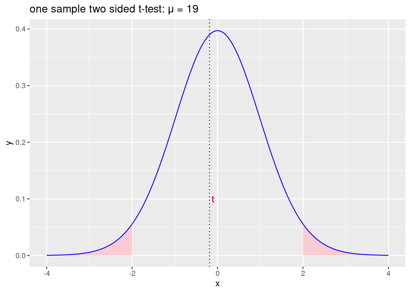

$Prihvaćamo početnu hipotezu $\mu =19$ i odbacujemo alternativnu hipotezu $\mu\neq19$$

Figure 2.2: Prihvaćamo početnu hipotezu $\mu =19$ i odbacujemo alternativnu hipotezu $\mu\neq19$

Jednosmjerni (less) t-test
Početna hipoteza: $\mu\geqslant21$
Alternativna hipoteza: $\mu<21$

rez1 <- t.test(x=ToothGrowth$len, mu = 21, alternative = "less")
rez1

## 
##  One Sample t-test
## 
## data:  ToothGrowth$len
## t = -2.2143, df = 59, p-value = 0.01534
## alternative hypothesis: true mean is less than 21
## 95 percent confidence interval:
##      -Inf 20.46358
## sample estimates:
## mean of x 
##  18.81333

Ručni izračun

mu <- 21
t = (Xbar - mu) / sbar
list(Xbar = Xbar,
     mu = mu,
     s = s,
     sbar = sbar,
     t = t,
     pvalue = pt(t, n-1),
     lower = -Inf,
     upper = Xbar - qt(0.05, df=n-1) * sbar)

## $Xbar
## [1] 18.81333
## 
## $mu
## [1] 21
## 
## $s
## [1] 7.649315
## 
## $sbar
## [1] 0.9875223
## 
## $t
## [1] -2.214296
## 
## $pvalue
## [1] 0.0153423
## 
## $lower
## [1] -Inf
## 
## $upper
## [1] 20.46358

tibble(x = seq(-4,4,0.01)) %>%
  ggplot(aes(x)) + 
  geom_text(aes(x=rez1$statistic, label="t", y=0.1), nudge_x = 0.08, colour="red",
            text=element_text(size=11)) +
  geom_area(stat = "function", fun = dt, args = list(df = n-1), fill = "pink", 
            xlim = c(-4, qt(0.05, df = n-1)), alpha=0.75) +
  geom_vline(xintercept = rez1$statistic, linetype = "dotted") +
  stat_function(fun=dt, args = list(df = n-1), color="blue") + 
  labs(title = "one sample less t-test: \u03BC \u2265 21")

$Odbacujemo početnu hipotezu $\mu\geqslant21$ i prihvaćamo alternativnu hipotezu $\mu<21$$

Figure 2.3: Odbacujemo početnu hipotezu $\mu\geqslant21$ i prihvaćamo alternativnu hipotezu $\mu<21$

Jednosmjerni (greater) t-test
Početna hipoteza: $\mu\leqslant21$
Alternativna hipoteza: $\mu>21$

rez2 <- t.test(x=ToothGrowth$len, mu = 21, alternative = "greater")
rez2

## 
##  One Sample t-test
## 
## data:  ToothGrowth$len
## t = -2.2143, df = 59, p-value = 0.9847
## alternative hypothesis: true mean is greater than 21
## 95 percent confidence interval:
##  17.16309      Inf
## sample estimates:
## mean of x 
##  18.81333

Ručni izračun

list(Xbar = Xbar,
     mu = mu,
     s = s,
     sbar = sbar,
     t = t,
     pvalue = pt(t, n-1, lower.tail = FALSE),
     lower = Xbar + qt(0.05, df=n-1) * sbar,
     upper = Inf)

## $Xbar
## [1] 18.81333
## 
## $mu
## [1] 21
## 
## $s
## [1] 7.649315
## 
## $sbar
## [1] 0.9875223
## 
## $t
## [1] -2.214296
## 
## $pvalue
## [1] 0.9846577
## 
## $lower
## [1] 17.16309
## 
## $upper
## [1] Inf

tibble(x = seq(-4,4,0.01)) %>%
  ggplot(aes(x)) + 
  geom_text(aes(x=rez2$statistic, label="t", y=0.1), nudge_x = 0.08, colour="red",
            text=element_text(size=11)) +
  geom_area(stat = "function", fun = dt, args = list(df = n-1), fill = "pink", 
            xlim = c(qt(0.95, df = n-1), 4), alpha=0.75) +
  geom_vline(xintercept = rez2$statistic, linetype = "dotted") +
  stat_function(fun=dt, args = list(df = n-1), color="blue") + 
  labs(title = "one sample greater t-test: \u03BC \u2264 21")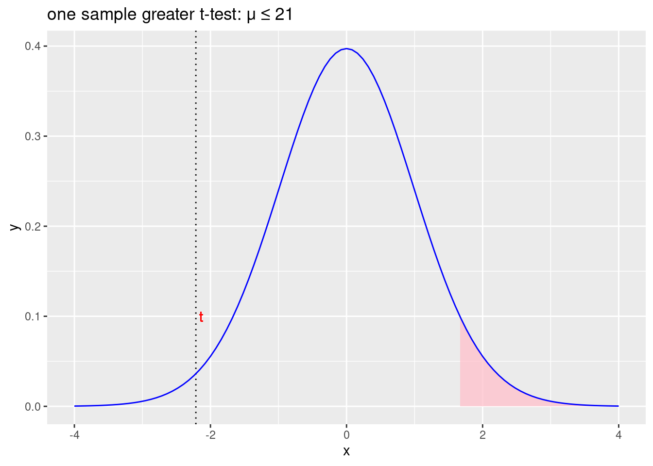

$Prihvaćamo početnu hipotezu $\mu\leqslant21$ i odbacujemo alternativnu hipotezu $\mu>21$$

Figure 2.4: Prihvaćamo početnu hipotezu $\mu\leqslant21$ i odbacujemo alternativnu hipotezu $\mu>21$

2.2 Two sample t-test for the difference in sample means

Question: Is the difference between the mean of two samples significantly different from zero?

When to use the test? You want to assess the extent to which the mean of two independent samples are different from each other. The test assumes the sample observations are normally distributed, and the sample variances are equal.

Dvosmjerni t-test
Početna hipoteza: $\mu_1=\mu_2$
Alternativna hipoteza: $\mu_1\neq\mu_2$

rez3 <- t.test(len ~ supp, data = ToothGrowth, var.equal = TRUE)
rez3

## 
##  Two Sample t-test
## 
## data:  len by supp
## t = 1.9153, df = 58, p-value = 0.06039
## alternative hypothesis: true difference in means between group OJ and group VC is not equal to 0
## 95 percent confidence interval:
##  -0.1670064  7.5670064
## sample estimates:
## mean in group OJ mean in group VC 
##         20.66333         16.96333

Ručni izračun

podaci <- ToothGrowth %>% group_by(supp) %>% 
  summarize(Xbar = mean(len), v = var(len), n = n())
s2_pool <- podaci %>% summarize(s2_pool = sum((n - 1) * v) / (sum(n) - 2)) %>% 
  pull(s2_pool)
Xbar <- podaci %>% pull(Xbar)
n <- podaci %>% pull(n)
SE <- sqrt(s2_pool * (1 / n[1] + 1 / n[2]))
t <- (Xbar[1] - Xbar[2]) / SE
list(podaci = podaci,
     pooled_variance = s2_pool,
     standard_error = SE,
     t = t,
     pvalue = ifelse(t < 0, 2*pt(t, sum(n)-2), 2*pt(t, sum(n)-2, lower.tail = FALSE)),
     lower = Xbar[1]-Xbar[2] + qt(0.025, df=sum(n)-2) * SE,
     upper = Xbar[1]-Xbar[2] - qt(0.025, df=sum(n)-2) * SE)

## $podaci
## # A tibble: 2 × 4
##   supp    Xbar      v     n
##   <fct>  <dbl>  <dbl> <int>
## 1 OJ    20.663 43.633    30
## 2 VC    16.963 68.327    30
## 
## $pooled_variance
## [1] 55.98033
## 
## $standard_error
## [1] 1.931844
## 
## $t
## [1] 1.915268
## 
## $pvalue
## [1] 0.06039337
## 
## $lower
## [1] -0.1670064
## 
## $upper
## [1] 7.567006

tibble(x = seq(-4,4,0.01)) %>%
  ggplot(aes(x)) + 
  geom_text(aes(x=rez3$statistic, label="t", y=0.1), nudge_x = 0.08, colour="red",
            text=element_text(size=11)) +
  geom_area(stat = "function", fun = dt, args = list(df = sum(n)-2), fill = "pink", 
            xlim = c(-4, qt(0.025, df = sum(n)-2)), alpha=0.75) +
  geom_area(stat = "function", fun = dt, args = list(df = sum(n)-2), fill = "pink", 
            xlim = c(qt(0.975, df = sum(n)-2), 4), alpha=0.75) +
  geom_vline(xintercept = rez3$statistic, linetype = "dotted") +
  stat_function(fun=dt, args = list(df = sum(n)-2), color="blue") + 
  labs(title = "two sample two sided t-test: \u03BC\u2081 = \u03BC\u2082")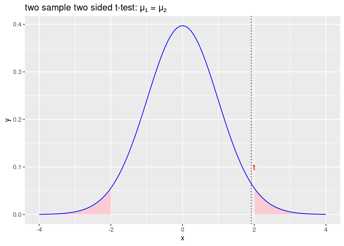

$Prihvaćamo početnu hipotezu $\mu_1 =\mu_2$ i odbacujemo alternativnu hipotezu $\mu_1\neq\mu_2$$

Figure 2.5: Prihvaćamo početnu hipotezu $\mu_1 =\mu_2$ i odbacujemo alternativnu hipotezu $\mu_1\neq\mu_2$

Jednosmjerni (less) t-test
Početna hipoteza: $\mu_1\geqslant\mu_2$
Alternativna hipoteza: $\mu_1<\mu_2$

rez4 <- t.test(len ~ supp, data = ToothGrowth, var.equal = TRUE, alternative = "less")
rez4

## 
##  Two Sample t-test
## 
## data:  len by supp
## t = 1.9153, df = 58, p-value = 0.9698
## alternative hypothesis: true difference in means between group OJ and group VC is less than 0
## 95 percent confidence interval:
##     -Inf 6.92918
## sample estimates:
## mean in group OJ mean in group VC 
##         20.66333         16.96333

Ručni izračun

list(podaci = podaci,
     pooled_variance = s2_pool,
     standard_error = SE,
     t = t,
     pvalue = pt(t, sum(n)-2),
     lower = -Inf,
     upper = Xbar[1]-Xbar[2] - qt(0.05, df=sum(n)-2) * SE)

## $podaci
## # A tibble: 2 × 4
##   supp    Xbar      v     n
##   <fct>  <dbl>  <dbl> <int>
## 1 OJ    20.663 43.633    30
## 2 VC    16.963 68.327    30
## 
## $pooled_variance
## [1] 55.98033
## 
## $standard_error
## [1] 1.931844
## 
## $t
## [1] 1.915268
## 
## $pvalue
## [1] 0.9698033
## 
## $lower
## [1] -Inf
## 
## $upper
## [1] 6.92918

tibble(x = seq(-4,4,0.01)) %>%
  ggplot(aes(x)) + 
  geom_text(aes(x=rez4$statistic, label="t", y=0.1), nudge_x = 0.08, colour="red",
            text=element_text(size=11)) +
  geom_area(stat = "function", fun = dt, args = list(df = sum(n)-2), fill = "pink", 
            xlim = c(-4, qt(0.05, df = sum(n)-2)), alpha=0.75) +
  geom_vline(xintercept = rez3$statistic, linetype = "dotted") +
  stat_function(fun=dt, args = list(df = sum(n)-2), color="blue") + 
  labs(title = "two sample less t-test: \u03BC\u2081 \u2265 \u03BC\u2082")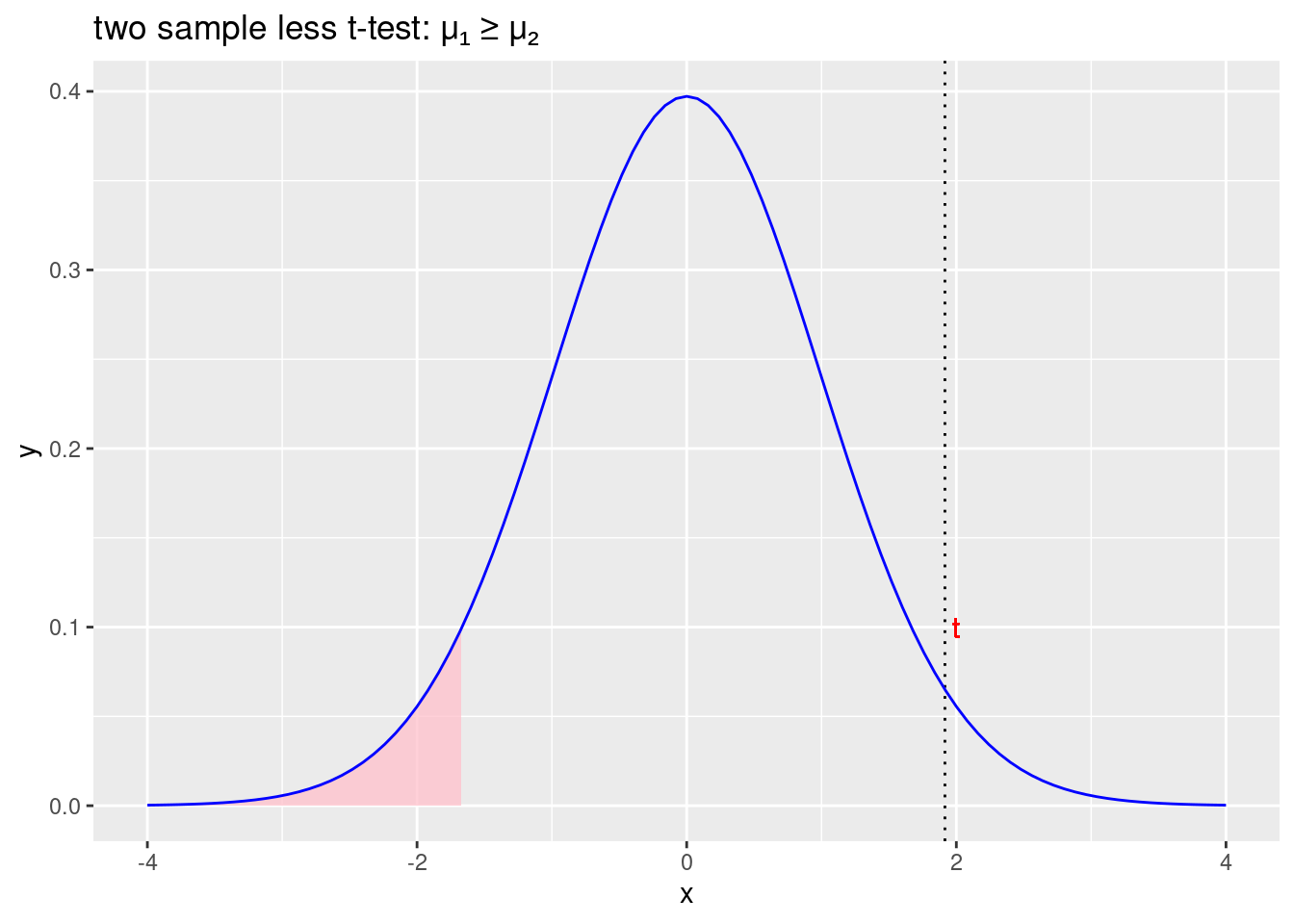

$Prihvaćamo početnu hipotezu $\mu_1\geqslant\mu_2$ i odbacujemo alternativnu hipotezu $\mu_1<\mu_2$$

Figure 2.6: Prihvaćamo početnu hipotezu $\mu_1\geqslant\mu_2$ i odbacujemo alternativnu hipotezu $\mu_1<\mu_2$

Jednosmjerni (greater) t-test
Početna hipoteza: $\mu_1\leqslant\mu_2$
Alternativna hipoteza: $\mu_1>\mu_2$

rez5 <- t.test(len ~ supp, data = ToothGrowth, var.equal = TRUE, alternative = "greater")
rez5

## 
##  Two Sample t-test
## 
## data:  len by supp
## t = 1.9153, df = 58, p-value = 0.0302
## alternative hypothesis: true difference in means between group OJ and group VC is greater than 0
## 95 percent confidence interval:
##  0.4708204       Inf
## sample estimates:
## mean in group OJ mean in group VC 
##         20.66333         16.96333

Ručni izračun

list(podaci = podaci,
     pooled_variance = s2_pool,
     standard_error = SE,
     t = t,
     pvalue = pt(t, sum(n)-2, lower.tail = FALSE),
     lower = Xbar[1]-Xbar[2] + qt(0.05, df=sum(n)-2) * SE,
     upper = Inf)

## $podaci
## # A tibble: 2 × 4
##   supp    Xbar      v     n
##   <fct>  <dbl>  <dbl> <int>
## 1 OJ    20.663 43.633    30
## 2 VC    16.963 68.327    30
## 
## $pooled_variance
## [1] 55.98033
## 
## $standard_error
## [1] 1.931844
## 
## $t
## [1] 1.915268
## 
## $pvalue
## [1] 0.03019669
## 
## $lower
## [1] 0.4708204
## 
## $upper
## [1] Inf

tibble(x = seq(-4,4,0.01)) %>%
  ggplot(aes(x)) + 
  geom_text(aes(x=rez5$statistic, label="t", y=0.1), nudge_x = 0.08, colour="red",
            text=element_text(size=11)) +
  geom_area(stat = "function", fun = dt, args = list(df = sum(n)-2), fill = "pink", 
            xlim = c(qt(0.95, df = sum(n)-2), 4), alpha=0.75) +
  geom_vline(xintercept = rez5$statistic, linetype = "dotted") +
  stat_function(fun=dt, args = list(df = sum(n)-2), color="blue") + 
  labs(title = "two sample greater t-test: \u03BC\u2081 \u2264 \u03BC\u2082")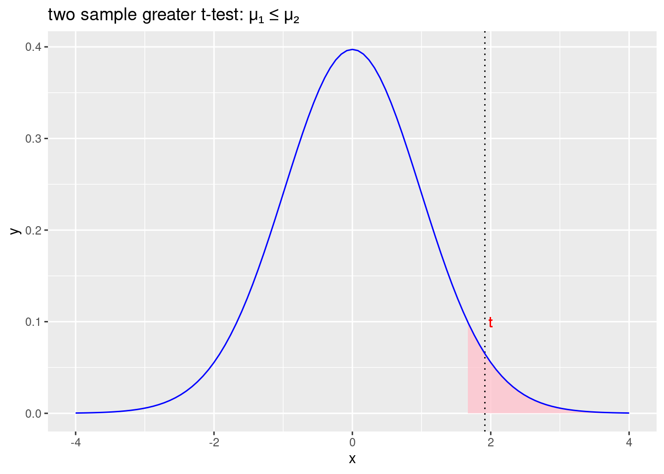

$Odbacujemo početnu hipotezu $\mu_1\leqslant\mu_2$ i prihvaćamo alternativnu hipotezu $\mu_1>\mu_2$$

Figure 2.7: Odbacujemo početnu hipotezu $\mu_1\leqslant\mu_2$ i prihvaćamo alternativnu hipotezu $\mu_1>\mu_2$

2.3 Welch t-test for the difference in sample means

Question: Is the difference between the mean of two samples significantly different from zero?

Dvosmjerni t-test
Početna hipoteza: $\mu_1=\mu_2$
Alternativna hipoteza: $\mu_1\neq\mu_2$

rez6 <- t.test(len ~ supp, data = ToothGrowth)
rez6

## 
##  Welch Two Sample t-test
## 
## data:  len by supp
## t = 1.9153, df = 55.309, p-value = 0.06063
## alternative hypothesis: true difference in means between group OJ and group VC is not equal to 0
## 95 percent confidence interval:
##  -0.1710156  7.5710156
## sample estimates:
## mean in group OJ mean in group VC 
##         20.66333         16.96333

Ručni izračun

podaci <- ToothGrowth %>% group_by(supp) %>% 
  summarize(Xbar = mean(len), v = var(len), n = n())
Xbar <- podaci %>% pull(Xbar)
SE <- podaci %>% summarize(SE = sqrt(sum(v / n))) %>% pull(SE)
t <- (Xbar[1] - Xbar[2]) / SE
degfr <- podaci %>% 
  summarize(degfr = sum(v / n)^2 / sum((v / n)^2 / (n - 1))) %>% 
  pull(degfr)
list(podaci = podaci,
     standard_error = SE,
     t = t,
     df = degfr,
     pvalue = ifelse(t < 0, 2*pt(t, degfr), 2*pt(t, degfr, lower.tail = FALSE)),
     lower = Xbar[1]-Xbar[2] + qt(0.025, df=degfr) * SE,
     upper = Xbar[1]-Xbar[2] - qt(0.025, df=degfr) * SE)

## $podaci
## # A tibble: 2 × 4
##   supp    Xbar      v     n
##   <fct>  <dbl>  <dbl> <int>
## 1 OJ    20.663 43.633    30
## 2 VC    16.963 68.327    30
## 
## $standard_error
## [1] 1.931844
## 
## $t
## [1] 1.915268
## 
## $df
## [1] 55.30943
## 
## $pvalue
## [1] 0.06063451
## 
## $lower
## [1] -0.1710156
## 
## $upper
## [1] 7.571016

tibble(x = seq(-4,4,0.01)) %>%
  ggplot(aes(x)) + 
  geom_text(aes(x=rez6$statistic, label="t", y=0.1), nudge_x = 0.08, colour="red",
            text=element_text(size=11)) +
  geom_area(stat = "function", fun = dt, args = list(df = degfr), fill = "pink", 
            xlim = c(-4, qt(0.025, df = degfr)), alpha=0.75) +
  geom_area(stat = "function", fun = dt, args = list(df = degfr), fill = "pink", 
            xlim = c(qt(0.975, df = degfr), 4), alpha=0.75) +
  geom_vline(xintercept = rez6$statistic, linetype = "dotted") +
  stat_function(fun=dt, args = list(df = degfr), color="blue") + 
  labs(title = "Welch two sample two sided t-test: \u03BC\u2081 = \u03BC\u2082")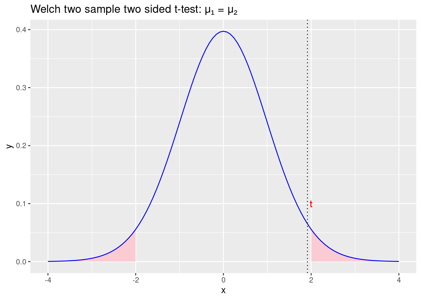

$Prihvaćamo početnu hipotezu $\mu_1 =\mu_2$ i odbacujemo alternativnu hipotezu $\mu_1\neq\mu_2$$

Figure 2.8: Prihvaćamo početnu hipotezu $\mu_1 =\mu_2$ i odbacujemo alternativnu hipotezu $\mu_1\neq\mu_2$

Jednosmjerni (less) t-test
Početna hipoteza: $\mu_1\geqslant\mu_2$
Alternativna hipoteza: $\mu_1<\mu_2$

rez7 <- t.test(len ~ supp, data = ToothGrowth, alternative = "less")
rez7

## 
##  Welch Two Sample t-test
## 
## data:  len by supp
## t = 1.9153, df = 55.309, p-value = 0.9697
## alternative hypothesis: true difference in means between group OJ and group VC is less than 0
## 95 percent confidence interval:
##      -Inf 6.931731
## sample estimates:
## mean in group OJ mean in group VC 
##         20.66333         16.96333

Ručni izračun

list(podaci = podaci,
     standard_error = SE,
     t = t,
     df = degfr,
     pvalue = pt(t, degfr),
     lower = -Inf,
     upper = Xbar[1]-Xbar[2] - qt(0.05, df=degfr) * SE)

## $podaci
## # A tibble: 2 × 4
##   supp    Xbar      v     n
##   <fct>  <dbl>  <dbl> <int>
## 1 OJ    20.663 43.633    30
## 2 VC    16.963 68.327    30
## 
## $standard_error
## [1] 1.931844
## 
## $t
## [1] 1.915268
## 
## $df
## [1] 55.30943
## 
## $pvalue
## [1] 0.9696827
## 
## $lower
## [1] -Inf
## 
## $upper
## [1] 6.931731

tibble(x = seq(-4,4,0.01)) %>%
  ggplot(aes(x)) + 
  geom_text(aes(x=rez7$statistic, label="t", y=0.1), nudge_x = 0.08, colour="red",
            text=element_text(size=11)) +
  geom_area(stat = "function", fun = dt, args = list(df = degfr), fill = "pink", 
            xlim = c(-4, qt(0.05, df = degfr)), alpha=0.75) +
  geom_vline(xintercept = rez7$statistic, linetype = "dotted") +
  stat_function(fun=dt, args = list(df = degfr), color="blue") + 
  labs(title = "Welch two sample less t-test: \u03BC\u2081 \u2265 \u03BC\u2082")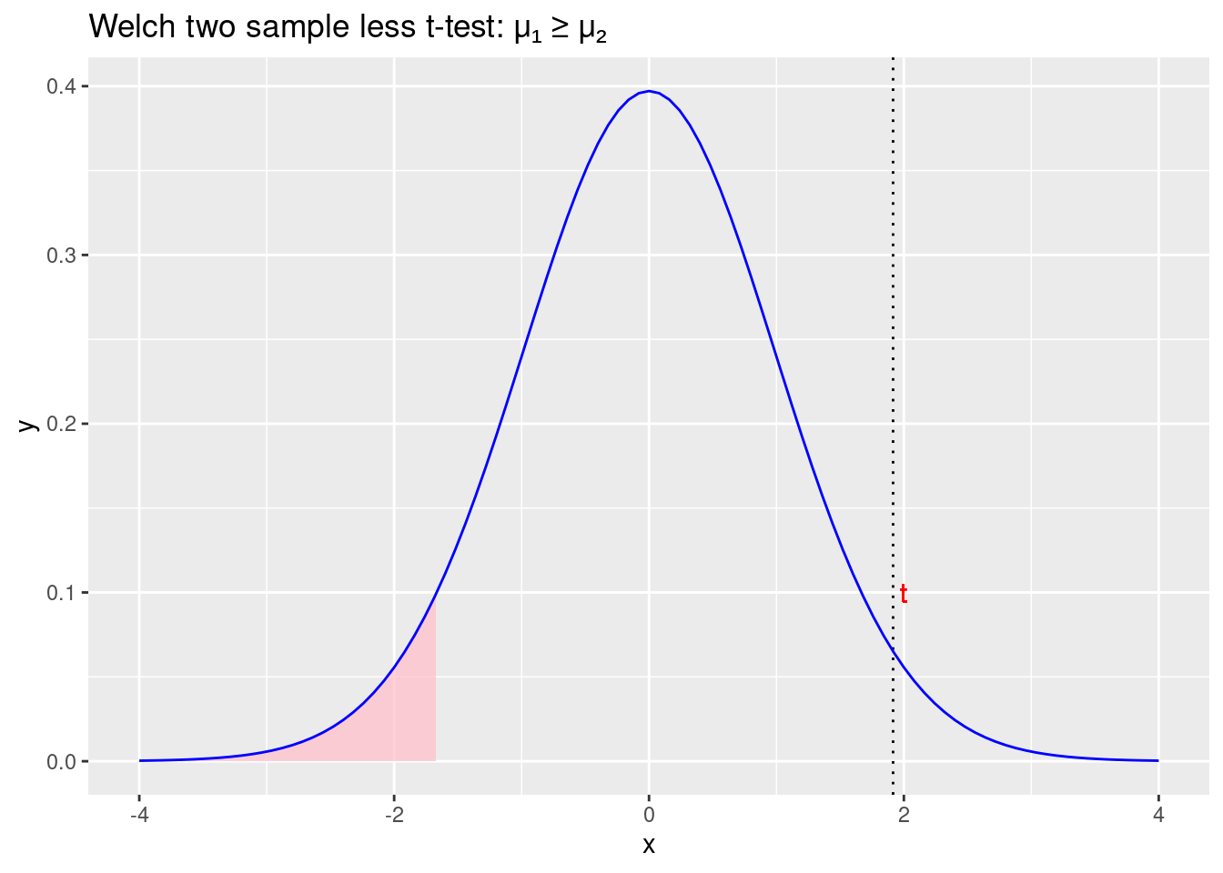

$Prihvaćamo početnu hipotezu $\mu_1 \geqslant\mu_2$ i odbacujemo alternativnu hipotezu $\mu_1<\mu_2$$

Figure 2.9: Prihvaćamo početnu hipotezu $\mu_1 \geqslant\mu_2$ i odbacujemo alternativnu hipotezu $\mu_1<\mu_2$

Jednosmjerni (greater) t-test
Početna hipoteza: $\mu_1\leqslant\mu_2$
Alternativna hipoteza: $\mu_1>\mu_2$

rez8 <- t.test(len ~ supp, data = ToothGrowth, alternative = "greater")
rez8

## 
##  Welch Two Sample t-test
## 
## data:  len by supp
## t = 1.9153, df = 55.309, p-value = 0.03032
## alternative hypothesis: true difference in means between group OJ and group VC is greater than 0
## 95 percent confidence interval:
##  0.4682687       Inf
## sample estimates:
## mean in group OJ mean in group VC 
##         20.66333         16.96333

Ručni izračun

list(podaci = podaci,
     standard_error = SE,
     t = t,
     df = degfr,
     pvalue = pt(t, degfr, lower.tail = FALSE),
     lower = Xbar[1]-Xbar[2] + qt(0.05, df=degfr) * SE,
     upper = Inf)

## $podaci
## # A tibble: 2 × 4
##   supp    Xbar      v     n
##   <fct>  <dbl>  <dbl> <int>
## 1 OJ    20.663 43.633    30
## 2 VC    16.963 68.327    30
## 
## $standard_error
## [1] 1.931844
## 
## $t
## [1] 1.915268
## 
## $df
## [1] 55.30943
## 
## $pvalue
## [1] 0.03031725
## 
## $lower
## [1] 0.4682687
## 
## $upper
## [1] Inf

tibble(x = seq(-4,4,0.01)) %>%
  ggplot(aes(x)) + 
  geom_text(aes(x=rez8$statistic, label="t", y=0.1), nudge_x = 0.08, colour="red",
            text=element_text(size=11)) +
  geom_area(stat = "function", fun = dt, args = list(df = degfr), fill = "pink", 
            xlim = c(qt(0.95, df = degfr), 4), alpha=0.75) +
  geom_vline(xintercept = rez8$statistic, linetype = "dotted") +
  stat_function(fun=dt, args = list(df = degfr), color="blue") + 
  labs(title = "Welch two sample greater t-test: \u03BC\u2081 \u2264 \u03BC\u2082")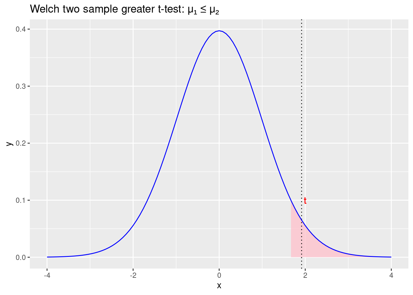

$Odbacujemo početnu hipotezu $\mu_1 \leqslant\mu_2$ i prihvaćamo alternativnu hipotezu $\mu_1>\mu_2$$

Figure 2.10: Odbacujemo početnu hipotezu $\mu_1 \leqslant\mu_2$ i prihvaćamo alternativnu hipotezu $\mu_1>\mu_2$

2.4 Paired t-test

Question: Is the difference between the mean of two samples significantly different from zero?

When to use the test? This test is used when each subject in a study is measured twice, before and after a treatment. Alternatively, in a matched pairs experimental design, where subjects are matched in pairs and different treatments are given to each subject pair. Subjects are assumed to be drawn from a population with a normal distribution.

Primjer

testovi <- tibble(test1 = c(16,20,21,22,23,22,27,25,27,28), 
                  test2 = c(19,22,24,24,25,25,26,26,28,32))

Dvosmjerni t-test
Početna hipoteza: $\mu=0$
Alternativna hipoteza: $\mu\neq0$

t.test(testovi$test2, testovi$test1, paired = TRUE)

## 
##  Paired t-test
## 
## data:  testovi$test2 and testovi$test1
## t = 4.4721, df = 9, p-value = 0.00155
## alternative hypothesis: true difference in means is not equal to 0
## 95 percent confidence interval:
##  0.9883326 3.0116674
## sample estimates:
## mean of the differences 
##                       2

Ručni izračun

n <- nrow(testovi)
razlika <- testovi$test2 - testovi$test1
Xbar <- mean(razlika)
s <- sd(razlika)
sbar <- s / sqrt(n)
t = Xbar / sbar
list(Xbar = Xbar,
     s = s,
     sbar = sbar,
     t = t,
     pvalue = ifelse(t < 0, 2*pt(t, n-1), 2*pt(t, n-1, lower.tail = FALSE)),
     lower = Xbar + qt(0.025, df=n-1) * sbar,
     upper = Xbar - qt(0.025, df=n-1) * sbar)

## $Xbar
## [1] 2
## 
## $s
## [1] 1.414214
## 
## $sbar
## [1] 0.4472136
## 
## $t
## [1] 4.472136
## 
## $pvalue
## [1] 0.001549886
## 
## $lower
## [1] 0.9883326
## 
## $upper
## [1] 3.011667

tibble(x = seq(-5,5,0.01)) %>%
  ggplot(aes(x)) + 
  geom_vline(xintercept = t, linetype = "dotted") +
  geom_text(aes(x=t, label="t", y=0.1), nudge_x = 0.1, colour="red",
            text=element_text(size=11)) +
  geom_area(stat = "function", fun = dt, args = list(df = n-1), fill = "pink", 
            xlim = c(-5, qt(0.025, df = n-1)), alpha=0.75) +
  geom_area(stat = "function", fun = dt, args = list(df = n-1), fill = "pink", 
            xlim = c(qt(0.975, df = n-1), 5), alpha=0.75) +
  stat_function(fun=dt, args = list(df = n-1), color="blue") + 
  labs(title = "paired two sided t-test: \u03BC = 0")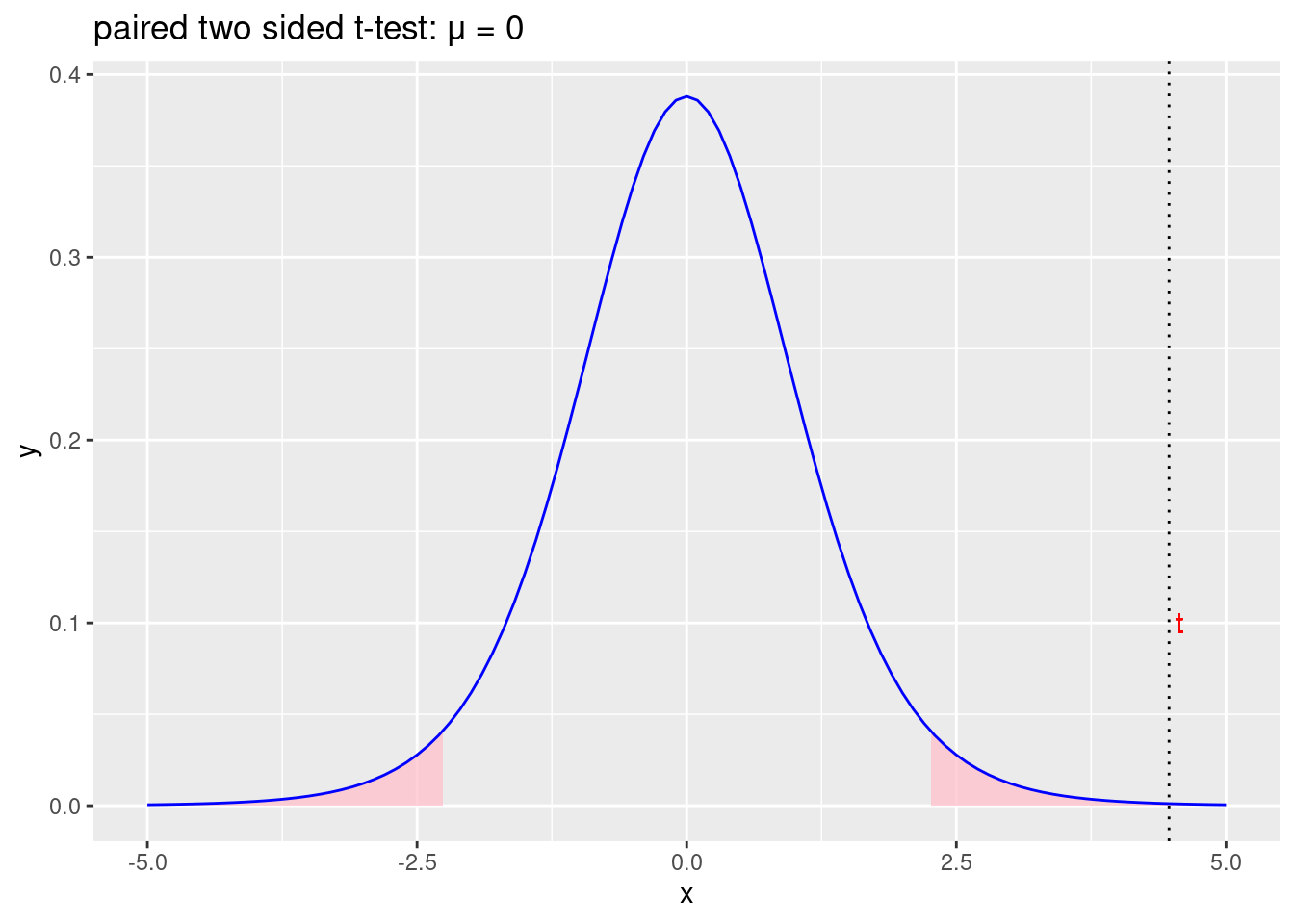

$Odbacujemo početnu hipotezu $\mu=0$ i prihvaćamo alternativnu hipotezu $\mu\neq0$$

Figure 2.11: Odbacujemo početnu hipotezu $\mu=0$ i prihvaćamo alternativnu hipotezu $\mu\neq0$

Jednosmjerni (less) t-test
Početna hipoteza: $\mu\geqslant0$
Alternativna hipoteza: $\mu<0$

t.test(testovi$test2, testovi$test1, alternative = "less", paired = TRUE)

## 
##  Paired t-test
## 
## data:  testovi$test2 and testovi$test1
## t = 4.4721, df = 9, p-value = 0.9992
## alternative hypothesis: true difference in means is less than 0
## 95 percent confidence interval:
##      -Inf 2.819793
## sample estimates:
## mean of the differences 
##                       2

Ručni izračun

list(Xbar = Xbar,
     s = s,
     sbar = sbar,
     t = t,
     pvalue = pt(t, n-1),
     lower = -Inf,
     upper = Xbar - qt(0.05, df=n-1) * sbar)

## $Xbar
## [1] 2
## 
## $s
## [1] 1.414214
## 
## $sbar
## [1] 0.4472136
## 
## $t
## [1] 4.472136
## 
## $pvalue
## [1] 0.9992251
## 
## $lower
## [1] -Inf
## 
## $upper
## [1] 2.819793

tibble(x = seq(-5,5,0.01)) %>%
  ggplot(aes(x)) + 
  geom_vline(xintercept = t, linetype = "dotted") +
  geom_text(aes(x=t, label="t", y=0.1), nudge_x = 0.1, colour="red",
            text=element_text(size=11)) +
  geom_area(stat = "function", fun = dt, args = list(df = n-1), fill = "pink", 
            xlim = c(-5, qt(0.05, df = n-1)), alpha=0.75) +
  stat_function(fun=dt, args = list(df = n-1), color="blue") + 
  labs(title = "paired less t-test: \u03BC \u2265 0")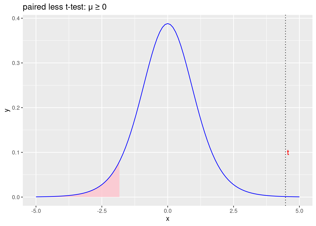

$Prihvaćamo početnu hipotezu $\mu\geqslant0$ i odbacujemo alternativnu hipotezu $\mu<0$$

Figure 2.12: Prihvaćamo početnu hipotezu $\mu\geqslant0$ i odbacujemo alternativnu hipotezu $\mu<0$

Jednosmjerni (greater) t-test
Početna hipoteza: $\mu\leqslant0$
Alternativna hipoteza: $\mu>0$

t.test(testovi$test2, testovi$test1, alternative = "greater", paired = TRUE)

## 
##  Paired t-test
## 
## data:  testovi$test2 and testovi$test1
## t = 4.4721, df = 9, p-value = 0.0007749
## alternative hypothesis: true difference in means is greater than 0
## 95 percent confidence interval:
##  1.180207      Inf
## sample estimates:
## mean of the differences 
##                       2

Ručni izračun

list(Xbar = Xbar,
     s = s,
     sbar = sbar,
     t = t,
     pvalue = pt(t, n-1, lower.tail = FALSE),
     lower = Xbar + qt(0.05, df=n-1) * sbar,
     upper = Inf)

## $Xbar
## [1] 2
## 
## $s
## [1] 1.414214
## 
## $sbar
## [1] 0.4472136
## 
## $t
## [1] 4.472136
## 
## $pvalue
## [1] 0.000774943
## 
## $lower
## [1] 1.180207
## 
## $upper
## [1] Inf

tibble(x = seq(-5,5,0.01)) %>%
  ggplot(aes(x)) + 
  geom_vline(xintercept = t, linetype = "dotted") +
  geom_text(aes(x=t, label="t", y=0.1), nudge_x = 0.1, colour="red",
            text=element_text(size=11)) +
  geom_area(stat = "function", fun = dt, args = list(df = n-1), fill = "pink", 
            xlim = c(qt(0.95, df = n-1), 5), alpha=0.75) +
  stat_function(fun=dt, args = list(df = n-1), color="blue") + 
  labs(title = "paired less t-test: \u03BC \u2264 0")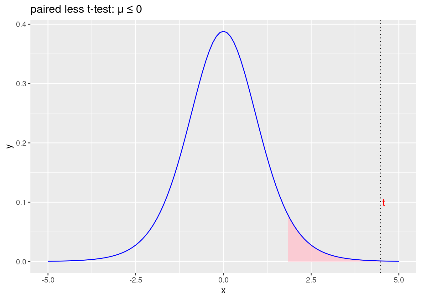

$Odbacujemo početnu hipotezu $\mu\leqslant0$ i prihvaćamo alternativnu hipotezu $\mu>0$$

Figure 2.13: Odbacujemo početnu hipotezu $\mu\leqslant0$ i prihvaćamo alternativnu hipotezu $\mu>0$

2.5 Two sample Wilcoxon test

Unlike the t-test, the Wilcoxon test doesn’t assume normality, which is nice. In fact, they don’t make any assumptions about what kind of distribution is involved: in statistical jargon, this makes them nonparametric tests. While avoiding the normality assumption is nice, there’s a drawback: the Wilcoxon test is usually less powerful than the t-test (i.e., higher Type II error rate).

Linkovi
Wilcoxon signed rank test, Wiki
Mann–Whitney U-test, Wiki
Mann–Whitney U-test, statskingdom

Question: Is the difference between the median of two samples significantly different from zero?

When to use the test? You want to assess the extent to which the median of two independent samples are different from each other. The test is less sensitive to outliers than the two sample t-test. Note, the test is some mes referred to as the Mann-Whitney U test, or the Mann-Whitney-Wilcoxon test.

Jedan primjer upotrebe gotove naredbe

wilcox.test(len ~ supp, data = ToothGrowth, alternative = "less", 
            exact = FALSE, correct = FALSE)

## 
##  Wilcoxon rank sum test
## 
## data:  len by supp
## W = 575.5, p-value = 0.9683
## alternative hypothesis: true location shift is less than 0

Ručni izračun

ToothGrowth %>% mutate(lenRank = rank(len)) %>% group_by(supp) %>% 
  summarize(R = sum(lenRank), n =n(), U = R - n * (n + 1) / 2)

## # A tibble: 2 × 4
##   supp       R     n     U
##   <fct>  <dbl> <int> <dbl>
## 1 OJ    1040.5    30 575.5
## 2 VC     789.5    30 324.5

tied <- table(rank(ToothGrowth$len))
tk <- sum(sapply(tied, function(x) x^3 - x))
n1 <- 30
n2 <- 30
n <- n1 + n2
pnorm(575.5, n1*n2/2, sqrt(n1 * n2 / 12 * (n + 1 - tk / (n*(n+1) ))))

## [1] 0.9682835

Rangovi

tibble(len = sort(ToothGrowth$len), len.rank = rank(len)) %>%
  print(n=Inf)

## # A tibble: 60 × 2
##      len len.rank
##    <dbl>    <dbl>
##  1   4.2      1  
##  2   5.2      2  
##  3   5.8      3  
##  4   6.4      4  
##  5   7        5  
##  6   7.3      6  
##  7   8.2      7  
##  8   9.4      8  
##  9   9.7      9.5
## 10   9.7      9.5
## 11  10       11.5
## 12  10       11.5
## 13  11.2     13.5
## 14  11.2     13.5
## 15  11.5     15  
## 16  13.6     16  
## 17  14.5     18  
## 18  14.5     18  
## 19  14.5     18  
## 20  15.2     20.5
## 21  15.2     20.5
## 22  15.5     22  
## 23  16.5     24  
## 24  16.5     24  
## 25  16.5     24  
## 26  17.3     26.5
## 27  17.3     26.5
## 28  17.6     28  
## 29  18.5     29  
## 30  18.8     30  
## 31  19.7     31  
## 32  20       32  
## 33  21.2     33  
## 34  21.5     34.5
## 35  21.5     34.5
## 36  22.4     36  
## 37  22.5     37  
## 38  23       38  
## 39  23.3     39.5
## 40  23.3     39.5
## 41  23.6     41.5
## 42  23.6     41.5
## 43  24.5     43  
## 44  24.8     44  
## 45  25.2     45  
## 46  25.5     46.5
## 47  25.5     46.5
## 48  25.8     48  
## 49  26.4     50.5
## 50  26.4     50.5
## 51  26.4     50.5
## 52  26.4     50.5
## 53  26.7     53  
## 54  27.3     54.5
## 55  27.3     54.5
## 56  29.4     56  
## 57  29.5     57  
## 58  30.9     58  
## 59  32.5     59  
## 60  33.9     60

2.6 One sample Wilcoxon test

Question: Is the median of a sample significantly different from a hypothesized value?

When to use the test? To test whether the median of sample is equal to a speciﬁed value. The null hypothesis is that the median of observations is zero (or some other speciﬁed value). It is a nonparametric test and therefore requires no assumption for the sample distribution. It is an alternative to the one-sample t-test when the normal assumption is not satisfied.

testovi <- tibble(test1 = c(16,20,21,22,23,22,27,25,27,28), 
                  test2 = c(19,22,24,24,25,25,26,26,28,32))

wilcox.test(testovi$test2, testovi$test1, paired = TRUE, alternative = "less")

## Warning in wilcox.test.default(testovi$test2, testovi$test1, paired = TRUE, :
## cannot compute exact p-value with ties

## 
##  Wilcoxon signed rank test with continuity correction
## 
## data:  testovi$test2 and testovi$test1
## V = 53, p-value = 0.9962
## alternative hypothesis: true location shift is less than 0

Literatura

Navarro, Daniel. 2015. Learning Statistics with R. https://learningstatisticswithr.com/book/index.html.